---
title: "Future snow | CliRSnow"
output: 
  flexdashboard::flex_dashboard:
    self_contained: false
    lib_dir: libs
    fig_mobile: false
    theme: bootstrap
    orientation: columns
    vertical_layout: fill
    social: menu
    source: embed
    logo: other/logo_72x48.png
    favicon: other/logo_72x48.png
    navbar:
      - { icon: "fa-share", title: "Main Dash", href: "./", align: right }
---

```{r setup, include=FALSE}
library(flexdashboard)
library(data.table)
library(forcats)
library(magrittr)
library(ggplot2)
library(flextable)

```


```{r, include=TRUE}
htmltools::tagList(fontawesome::fa_html_dependency())
```


```{r data-prep-summary}
load(here::here("data/future-summary-elev-500m.rda"))


setnames(dat_bc, "alt_f", "elev_f")
dat_bc[, elev := tstrsplit(elev_f, ",") %>% sapply(readr::parse_number) %>% rowMeans]
dat_ds[, elev := tstrsplit(elev_f, ",") %>% sapply(readr::parse_number) %>% rowMeans]

dat_ens_mean <- dat_ds[elev > 200 & elev < 3600,
                       .(scd = round(mean(scd))),
                       .(elev_f, elev, experiment, period, fp)]


# dat_ens_mean <- dat_bc[elev > 200 & elev < 3600,
#                        .(scd = mean(snc)*365),
#                        .(elev_f, elev, experiment, period, fp)]

dat_ens_mean[, period_f := fct_recode(period,
                                      "2001\n-\n2020" = "2001-2020",
                                      "2041\n-\n2070" = "2041-2070",
                                      "2071\n-\n2100" = "2071-2100")]

dat_ens_mean[period != "2041-2070"] %>% 
  dcast(elev ~ experiment + fp, value.var = "scd") -> dat_lollipop

dat_lollipop[, elev_fct := fct_inorder(paste0(elev, " m"))]

dat_lollipop[, .(elev,
                 v1 = rcp85_future, 
                 v2 = rcp26_future - rcp85_future,
                 v3 = rcp26_past - rcp26_future)] %>% 
  melt(id.vars = "elev",
       measure.vars = paste0("v", 1:3)) %>% 
  .[,
    .(i_dot_grp = 1:round(value)),
    .(elev, variable)] -> dat_dp


dat_dp[, i_dot := 1:.N - 1, elev]
dat_dp[, xx := i_dot %% 10]
dat_dp[, yy := i_dot %/% 10]

x_rat <- 80
elev_plot <- c(500, 1500, 2500, 3500)

dat_dp[, xx_plot := elev + x_rat*xx - 9*x_rat/2]


dat_text <- dat_lollipop[elev %in% elev_plot,
                         .(elev, 
                           yy = ceiling(rcp26_past/10) + 1.5, 
                           past = round(rcp26_past),
                           loss = round(rcp26_past - rcp26_future),
                           climact = round(rcp26_future - rcp85_future))]
dat_text[, past_ch := sprintf("%6s", past)]
dat_text[, loss_ch := sprintf("%5s", loss)]
dat_text[, climact_ch := sprintf("%5s", climact)]

```





# Summary

## Column {.tabset .tabset-fade}

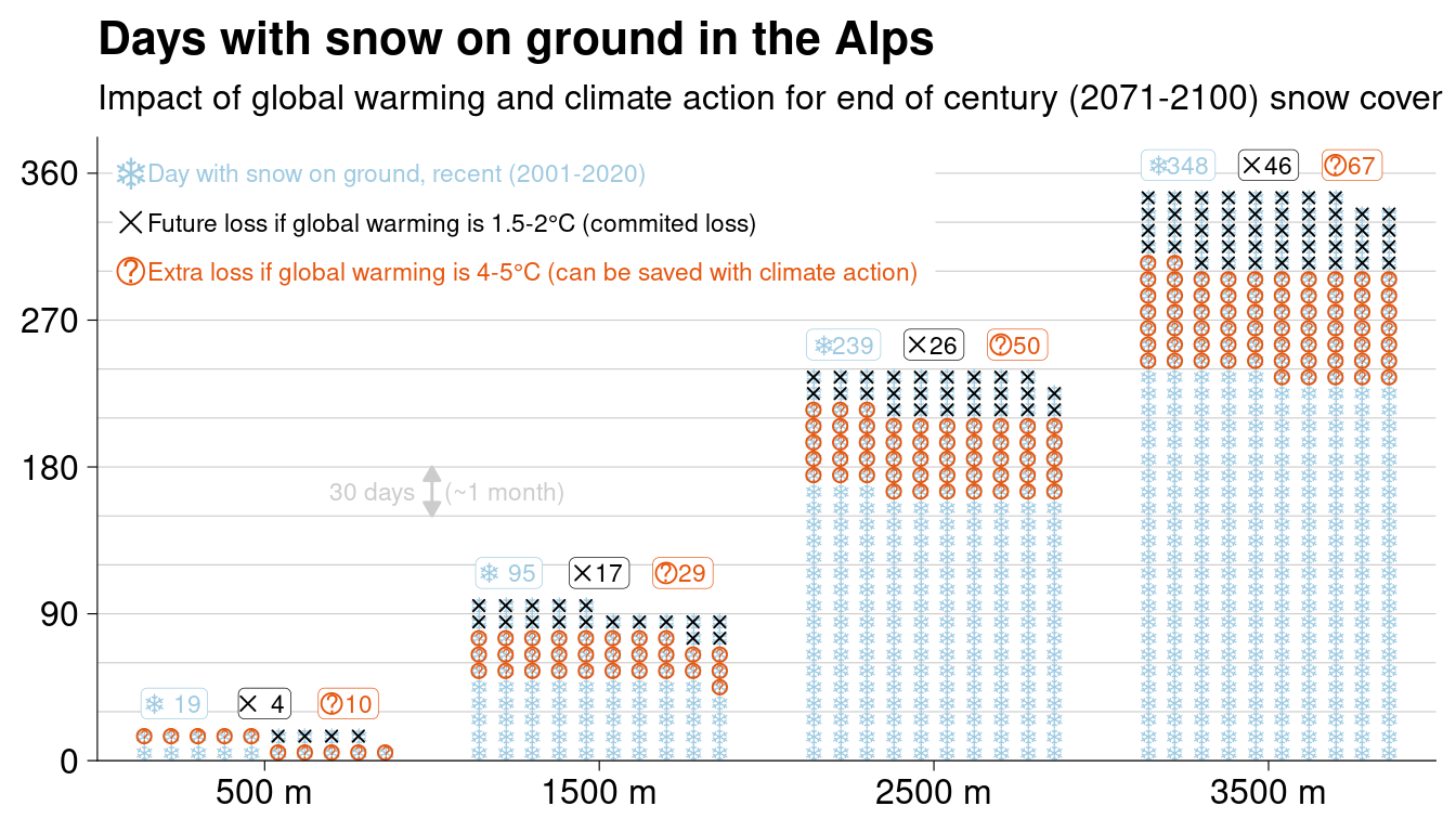
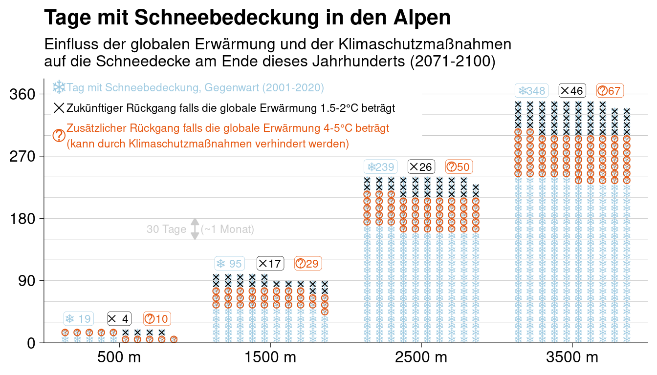
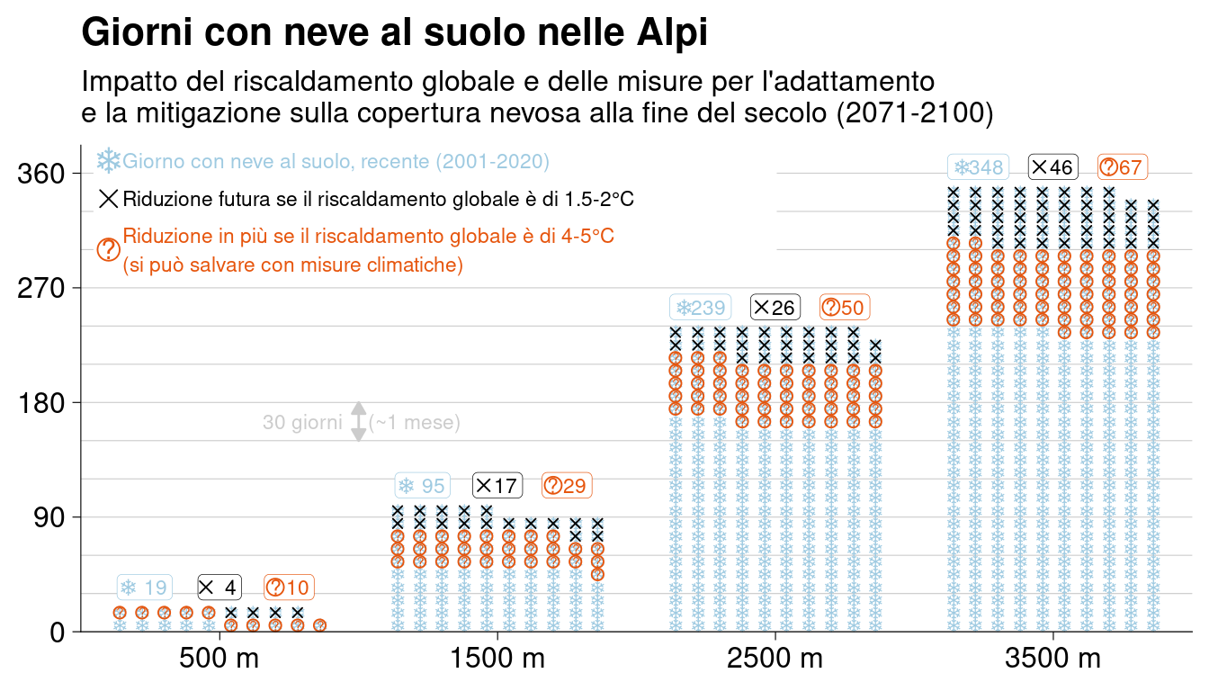
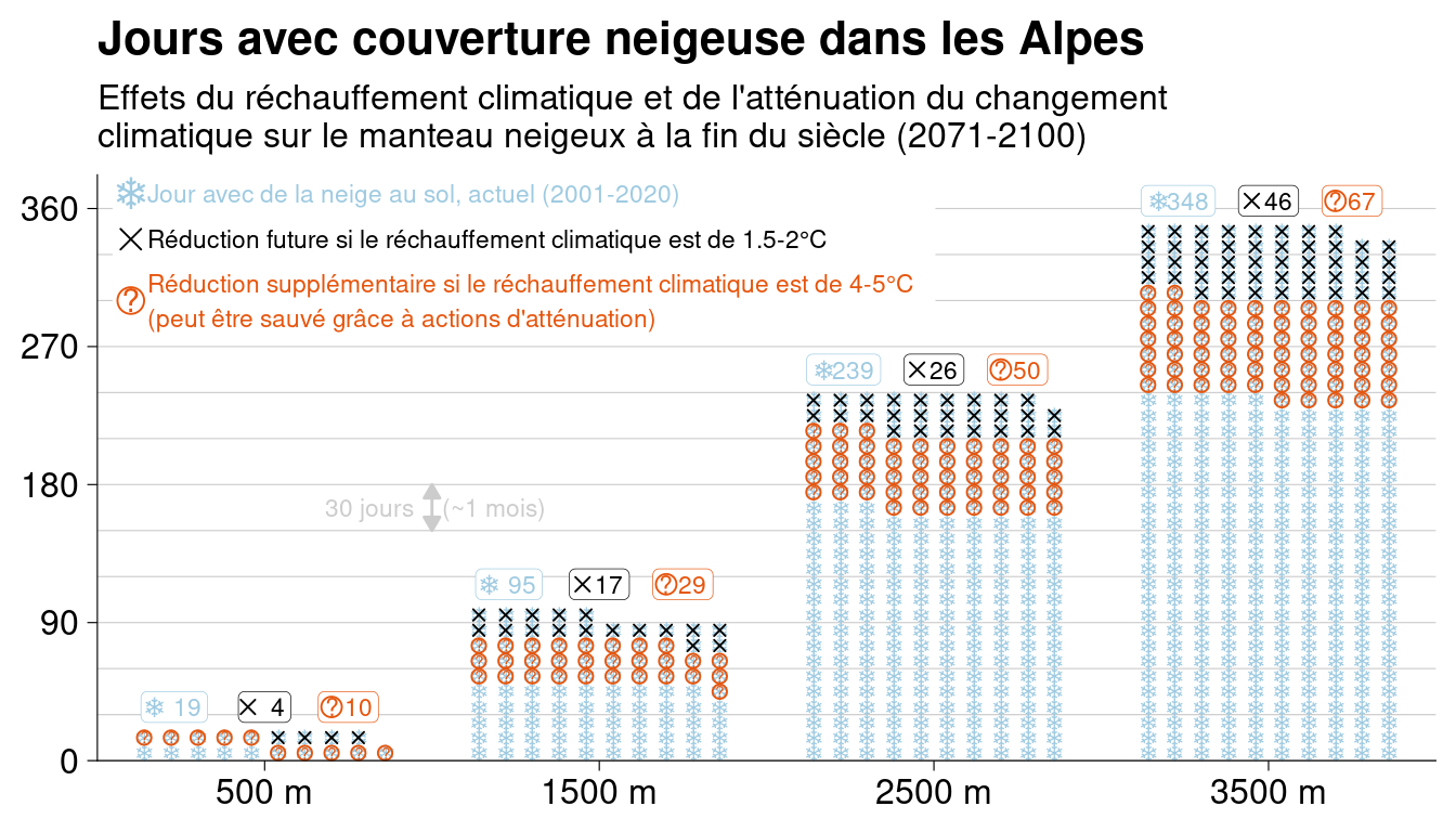
> What can be saved? The impact of climate action on 21st century snow cover duration in the Alps.

### English

```{r fig.width=7, fig.height=4}


dat_dp[elev %in% elev_plot] %>% 
  ggplot(aes(xx_plot, yy+0.5))+
  geom_hline(yintercept = 0:12*3, colour = grey(0.8), size = 0.2)+ # 1 month
  
  geom_point(shape = "\u2744", size = 2.5, colour = "#9ecae1")+
  geom_point(data = dat_dp[elev %in% elev_plot & variable == "v3"] ,
             shape = 4, size = 1.5, colour = "black")+
  geom_point(data = dat_dp[elev %in% elev_plot & variable == "v2"] ,
             shape = 1, size = 2, colour = "#e6550d")+
  geom_text(data = dat_dp[elev %in% elev_plot & variable == "v2"] ,
            label = "?", fontface = "plain", size = 2, colour = "#e6550d")+
  cowplot::theme_cowplot(line_size = 0.2)+
  theme(plot.background = element_rect(colour = "white", fill = "white"))+
  scale_x_continuous(NULL, limits = c(0, 4000), expand = c(0,0),
                     breaks = elev_plot, labels = paste0(elev_plot, " m"))+
  # scale_y_continuous(NULL, breaks = c(0,10,20,30), labels = c(0,10,20,30)*10)+
  scale_y_continuous(NULL, limits = c(0, 36.2 + 2), expand = c(0,0),
                     breaks = c(0,9,18,27,36), labels = c(0,9,18,27,36)*10)+
  ggtitle("Days with snow on ground in the Alps",
          "Impact of global warming and climate action for end of century (2071-2100) snow cover")+
  
  #legend
  annotate("rect", xmin = 50, xmax = 2500, ymin = 28.5, ymax = 37.5, 
           colour = "white", fill = "white")+
  annotate("point", 100, 36, shape = "\u2744", size = 5, colour = "#9ecae1")+
  annotate("text", 150, 36, hjust = 0, vjust = 0.5, size = 3, 
           label = "Day with snow on ground, recent (2001-2020)", colour = "#9ecae1")+
  
  annotate("point", 100, 33, shape = 4, size = 3, colour = "black")+
  annotate("text", 150, 33, hjust = 0, vjust = 0.5, size = 3, 
           label = "Future loss if global warming is 1.5-2°C (commited loss)", colour = "black")+
  
  annotate("point", 100, 30, shape = 1, size = 4, colour = "#e6550d")+
  annotate("text", 100, 30, label = "?", fontface = "plain", size = 4, colour = "#e6550d")+
  annotate("text", 150, 30, hjust = 0, vjust = 0.5, size = 3,
           label = "Extra loss if global warming is 4-5°C (can be saved with climate action)",
           colour = "#e6550d")+
  
  # grid stuff
  annotate("segment", x = 1000, xend = 1000, y = 18, yend = 15, colour = grey(0.8),
           arrow = arrow(ends = "both", type = "closed", length = unit(0.075, "in")))+
  annotate("text", x = 1000, y = 16.5, hjust = -0.1, size = 3,
           label = "(~1 month)", colour = grey(0.8))+
  annotate("text", x = 1000, y = 16.5, hjust = 1.2, size = 3,
           label = "30 days", colour = grey(0.8))+
  
  # text
  geom_label(data = dat_text, 
            aes(elev - 270, yy, label = past_ch),
            hjust = 0.5, vjust = 0.5, colour = "#9ecae1", size = 3, 
            label.padding = unit(0.15, "lines"), label.size = 0.12)+
  geom_point(data = dat_text, 
             aes(elev - 270 - 60, yy),
             shape = "\u2744", size = 3, colour = "#9ecae1")+
  geom_label(data = dat_text, 
             aes(elev, yy, label = loss_ch),
             hjust = 0.5, vjust = 0.5, colour = "black", size = 3,
             label.padding = unit(0.15, "lines"), label.size = 0.12)+
  geom_point(data = dat_text, 
             aes(elev - 50, yy),
             shape = 4, size = 2, colour = "black")+
  geom_label(data = dat_text, 
             aes(elev + 250, yy, label = climact_ch),
             hjust = 0.5, vjust = 0.5, colour = "#e6550d", size = 3,
             label.padding = unit(0.15, "lines"), label.size = 0.12)+
  geom_point(data = dat_text, 
             aes(elev + 250 - 50, yy),
             shape = 1, size = 3, colour = "#e6550d")+
  geom_text(data = dat_text, 
            aes(elev + 250 - 50, yy, label = "?"),
            size = 3, colour = "#e6550d")

```


### Deutsch

```{r fig.width=7, fig.height=4}


dat_dp[elev %in% elev_plot] %>% 
  ggplot(aes(xx_plot, yy+0.5))+
  geom_hline(yintercept = 0:12*3, colour = grey(0.8), size = 0.2)+ # 1 month
  
  geom_point(shape = "\u2744", size = 2.5, colour = "#9ecae1")+
  geom_point(data = dat_dp[elev %in% elev_plot & variable == "v3"] ,
             shape = 4, size = 1.5, colour = "black")+
  geom_point(data = dat_dp[elev %in% elev_plot & variable == "v2"] ,
             shape = 1, size = 2, colour = "#e6550d")+
  geom_text(data = dat_dp[elev %in% elev_plot & variable == "v2"] ,
            label = "?", fontface = "plain", size = 2, colour = "#e6550d")+
  cowplot::theme_cowplot(line_size = 0.2)+
  theme(plot.background = element_rect(colour = "white", fill = "white"))+
  scale_x_continuous(NULL, limits = c(0, 4000), expand = c(0,0),
                     breaks = elev_plot, labels = paste0(elev_plot, " m"))+
  # scale_y_continuous(NULL, breaks = c(0,10,20,30), labels = c(0,10,20,30)*10)+
  scale_y_continuous(NULL, limits = c(0, 36.2 + 2), expand = c(0,0),
                     breaks = c(0,9,18,27,36), labels = c(0,9,18,27,36)*10)+
  ggtitle("Tage mit Schneebedeckung in den Alpen",
          "Einfluss der globalen Erwärmung und der Klimaschutzmaßnahmen \nauf die Schneedecke am Ende dieses Jahrhunderts (2071-2100)")+
  
  #legend
  annotate("rect", xmin = 50, xmax = 2500, ymin = 28.5, ymax = 37.5, 
           colour = "white", fill = "white")+
  annotate("point", 100, 36+1, shape = "\u2744", size = 5, colour = "#9ecae1")+
  annotate("text", 150, 36+1, hjust = 0, vjust = 0.5, size = 3, 
           label = "Tag mit Schneebedeckung, Gegenwart (2001-2020)", colour = "#9ecae1")+
  
  annotate("point", 100, 33+1, shape = 4, size = 3, colour = "black")+
  annotate("text", 150, 33+1, hjust = 0, vjust = 0.5, size = 3, 
           label = "Zukünftiger Rückgang falls die globale Erwärmung 1.5-2°C beträgt", colour = "black")+
  
  annotate("point", 100, 30, shape = 1, size = 4, colour = "#e6550d")+
  annotate("text", 100, 30, label = "?", fontface = "plain", size = 4, colour = "#e6550d")+
  annotate("text", 150, 30, hjust = 0, vjust = 0.5, size = 3,
           label = "Zusätzlicher Rückgang falls die globale Erwärmung 4-5°C beträgt\n(kann durch Klimaschutzmaßnahmen verhindert werden)",
           colour = "#e6550d")+
  
  # grid stuff
  annotate("segment", x = 1000, xend = 1000, y = 18, yend = 15, colour = grey(0.8),
           arrow = arrow(ends = "both", type = "closed", length = unit(0.075, "in")))+
  annotate("text", x = 1000, y = 16.5, hjust = -0.1, size = 3,
           label = "(~1 Monat)", colour = grey(0.8))+
  annotate("text", x = 1000, y = 16.5, hjust = 1.2, size = 3,
           label = "30 Tage", colour = grey(0.8))+
  
  # text
  geom_label(data = dat_text, 
             aes(elev - 270, yy, label = past_ch),
             hjust = 0.5, vjust = 0.5, colour = "#9ecae1", size = 3, 
             label.padding = unit(0.15, "lines"), label.size = 0.12)+
  geom_point(data = dat_text, 
             aes(elev - 270 - 60, yy),
             shape = "\u2744", size = 3, colour = "#9ecae1")+
  geom_label(data = dat_text, 
             aes(elev, yy, label = loss_ch),
             hjust = 0.5, vjust = 0.5, colour = "black", size = 3,
             label.padding = unit(0.15, "lines"), label.size = 0.12)+
  geom_point(data = dat_text, 
             aes(elev - 50, yy),
             shape = 4, size = 2, colour = "black")+
  geom_label(data = dat_text, 
             aes(elev + 250, yy, label = climact_ch),
             hjust = 0.5, vjust = 0.5, colour = "#e6550d", size = 3,
             label.padding = unit(0.15, "lines"), label.size = 0.12)+
  geom_point(data = dat_text, 
             aes(elev + 250 - 50, yy),
             shape = 1, size = 3, colour = "#e6550d")+
  geom_text(data = dat_text, 
            aes(elev + 250 - 50, yy, label = "?"),
            size = 3, colour = "#e6550d")

```


### Italiano

```{r fig.width=7, fig.height=4}


dat_dp[elev %in% elev_plot] %>% 
  ggplot(aes(xx_plot, yy+0.5))+
  geom_hline(yintercept = 0:12*3, colour = grey(0.8), size = 0.2)+ # 1 month
  
  geom_point(shape = "\u2744", size = 2.5, colour = "#9ecae1")+
  geom_point(data = dat_dp[elev %in% elev_plot & variable == "v3"] ,
             shape = 4, size = 1.5, colour = "black")+
  geom_point(data = dat_dp[elev %in% elev_plot & variable == "v2"] ,
             shape = 1, size = 2, colour = "#e6550d")+
  geom_text(data = dat_dp[elev %in% elev_plot & variable == "v2"] ,
            label = "?", fontface = "plain", size = 2, colour = "#e6550d")+
  cowplot::theme_cowplot(line_size = 0.2)+
  theme(plot.background = element_rect(colour = "white", fill = "white"))+
  scale_x_continuous(NULL, limits = c(0, 4000), expand = c(0,0),
                     breaks = elev_plot, labels = paste0(elev_plot, " m"))+
  # scale_y_continuous(NULL, breaks = c(0,10,20,30), labels = c(0,10,20,30)*10)+
  scale_y_continuous(NULL, limits = c(0, 36.2 + 2), expand = c(0,0),
                     breaks = c(0,9,18,27,36), labels = c(0,9,18,27,36)*10)+
  ggtitle("Giorni con neve al suolo nelle Alpi",
          "Impatto del riscaldamento globale e delle misure per l'adattamento \ne la mitigazione sulla copertura nevosa alla fine del secolo (2071-2100)")+
  
  #legend
  annotate("rect", xmin = 50, xmax = 2500, ymin = 28.5, ymax = 37.5, 
           colour = "white", fill = "white")+
  annotate("point", 100, 36+1, shape = "\u2744", size = 5, colour = "#9ecae1")+
  annotate("text", 150, 36+1, hjust = 0, vjust = 0.5, size = 3, 
           label = "Giorno con neve al suolo, recente (2001-2020)", colour = "#9ecae1")+
  
  annotate("point", 100, 33+1, shape = 4, size = 3, colour = "black")+
  annotate("text", 150, 33+1, hjust = 0, vjust = 0.5, size = 3, 
           label = "Riduzione futura se il riscaldamento globale è di 1.5-2°C", colour = "black")+
  
  annotate("point", 100, 30, shape = 1, size = 4, colour = "#e6550d")+
  annotate("text", 100, 30, label = "?", fontface = "plain", size = 4, colour = "#e6550d")+
  annotate("text", 150, 30, hjust = 0, vjust = 0.5, size = 3,
           label = "Riduzione in più se il riscaldamento globale è di 4-5°C\n(si può salvare con misure climatiche)",
           colour = "#e6550d")+
  
  # grid stuff
  annotate("segment", x = 1000, xend = 1000, y = 18, yend = 15, colour = grey(0.8),
           arrow = arrow(ends = "both", type = "closed", length = unit(0.075, "in")))+
  annotate("text", x = 1000, y = 16.5, hjust = -0.1, size = 3,
           label = "(~1 mese)", colour = grey(0.8))+
  annotate("text", x = 1000, y = 16.5, hjust = 1.2, size = 3,
           label = "30 giorni", colour = grey(0.8))+
  
  # text
  geom_label(data = dat_text, 
             aes(elev - 270, yy, label = past_ch),
             hjust = 0.5, vjust = 0.5, colour = "#9ecae1", size = 3, 
             label.padding = unit(0.15, "lines"), label.size = 0.12)+
  geom_point(data = dat_text, 
             aes(elev - 270 - 60, yy),
             shape = "\u2744", size = 3, colour = "#9ecae1")+
  geom_label(data = dat_text, 
             aes(elev, yy, label = loss_ch),
             hjust = 0.5, vjust = 0.5, colour = "black", size = 3,
             label.padding = unit(0.15, "lines"), label.size = 0.12)+
  geom_point(data = dat_text, 
             aes(elev - 50, yy),
             shape = 4, size = 2, colour = "black")+
  geom_label(data = dat_text, 
             aes(elev + 250, yy, label = climact_ch),
             hjust = 0.5, vjust = 0.5, colour = "#e6550d", size = 3,
             label.padding = unit(0.15, "lines"), label.size = 0.12)+
  geom_point(data = dat_text, 
             aes(elev + 250 - 50, yy),
             shape = 1, size = 3, colour = "#e6550d")+
  geom_text(data = dat_text, 
            aes(elev + 250 - 50, yy, label = "?"),
            size = 3, colour = "#e6550d")

```

### Français

```{r fig.width=7, fig.height=4}


dat_dp[elev %in% elev_plot] %>% 
  ggplot(aes(xx_plot, yy+0.5))+
  geom_hline(yintercept = 0:12*3, colour = grey(0.8), size = 0.2)+ # 1 month
  
  geom_point(shape = "\u2744", size = 2.5, colour = "#9ecae1")+
  geom_point(data = dat_dp[elev %in% elev_plot & variable == "v3"] ,
             shape = 4, size = 1.5, colour = "black")+
  geom_point(data = dat_dp[elev %in% elev_plot & variable == "v2"] ,
             shape = 1, size = 2, colour = "#e6550d")+
  geom_text(data = dat_dp[elev %in% elev_plot & variable == "v2"] ,
            label = "?", fontface = "plain", size = 2, colour = "#e6550d")+
  cowplot::theme_cowplot(line_size = 0.2)+
  theme(plot.background = element_rect(colour = "white", fill = "white"))+
  scale_x_continuous(NULL, limits = c(0, 4000), expand = c(0,0),
                     breaks = elev_plot, labels = paste0(elev_plot, " m"))+
  # scale_y_continuous(NULL, breaks = c(0,10,20,30), labels = c(0,10,20,30)*10)+
  scale_y_continuous(NULL, limits = c(0, 36.2 + 2), expand = c(0,0),
                     breaks = c(0,9,18,27,36), labels = c(0,9,18,27,36)*10)+
  ggtitle("Jours avec couverture neigeuse dans les Alpes",
          "Effets du réchauffement climatique et de l'atténuation du changement\nclimatique sur le manteau neigeux à la fin du siècle (2071-2100)")+
  
  #legend
  annotate("rect", xmin = 50, xmax = 2500, ymin = 28.5, ymax = 37.5, 
           colour = "white", fill = "white")+
  annotate("point", 100, 36+1, shape = "\u2744", size = 5, colour = "#9ecae1")+
  annotate("text", 150, 36+1, hjust = 0, vjust = 0.5, size = 3, 
           label = "Jour avec de la neige au sol, actuel (2001-2020)", colour = "#9ecae1")+
  
  annotate("point", 100, 33+1, shape = 4, size = 3, colour = "black")+
  annotate("text", 150, 33+1, hjust = 0, vjust = 0.5, size = 3, 
           label = "Réduction future si le réchauffement climatique est de 1.5-2°C", colour = "black")+
  
  annotate("point", 100, 30, shape = 1, size = 4, colour = "#e6550d")+
  annotate("text", 100, 30, label = "?", fontface = "plain", size = 4, colour = "#e6550d")+
  annotate("text", 150, 30, hjust = 0, vjust = 0.5, size = 3,
           label = "Réduction supplémentaire si le réchauffement climatique est de 4-5°C \n(peut être sauvé grâce à actions d'atténuation)",
           colour = "#e6550d")+
  
  # grid stuff
  annotate("segment", x = 1000, xend = 1000, y = 18, yend = 15, colour = grey(0.8),
           arrow = arrow(ends = "both", type = "closed", length = unit(0.075, "in")))+
  annotate("text", x = 1000, y = 16.5, hjust = -0.1, size = 3,
           label = "(~1 mois)", colour = grey(0.8))+
  annotate("text", x = 1000, y = 16.5, hjust = 1.2, size = 3,
           label = "30 jours", colour = grey(0.8))+
  
  # text
  geom_label(data = dat_text, 
             aes(elev - 270, yy, label = past_ch),
             hjust = 0.5, vjust = 0.5, colour = "#9ecae1", size = 3, 
             label.padding = unit(0.15, "lines"), label.size = 0.12)+
  geom_point(data = dat_text, 
             aes(elev - 270 - 60, yy),
             shape = "\u2744", size = 3, colour = "#9ecae1")+
  geom_label(data = dat_text, 
             aes(elev, yy, label = loss_ch),
             hjust = 0.5, vjust = 0.5, colour = "black", size = 3,
             label.padding = unit(0.15, "lines"), label.size = 0.12)+
  geom_point(data = dat_text, 
             aes(elev - 50, yy),
             shape = 4, size = 2, colour = "black")+
  geom_label(data = dat_text, 
             aes(elev + 250, yy, label = climact_ch),
             hjust = 0.5, vjust = 0.5, colour = "#e6550d", size = 3,
             label.padding = unit(0.15, "lines"), label.size = 0.12)+
  geom_point(data = dat_text, 
             aes(elev + 250 - 50, yy),
             shape = 1, size = 3, colour = "#e6550d")+
  geom_text(data = dat_text, 
            aes(elev + 250 - 50, yy, label = "?"),
            size = 3, colour = "#e6550d")

```


### Español

```{r fig.width=7, fig.height=4}


dat_dp[elev %in% elev_plot] %>% 
  ggplot(aes(xx_plot, yy+0.5))+
  geom_hline(yintercept = 0:12*3, colour = grey(0.8), size = 0.2)+ # 1 month
  
  geom_point(shape = "\u2744", size = 2.5, colour = "#9ecae1")+
  geom_point(data = dat_dp[elev %in% elev_plot & variable == "v3"] ,
             shape = 4, size = 1.5, colour = "black")+
  geom_point(data = dat_dp[elev %in% elev_plot & variable == "v2"] ,
             shape = 1, size = 2, colour = "#e6550d")+
  geom_text(data = dat_dp[elev %in% elev_plot & variable == "v2"] ,
            label = "?", fontface = "plain", size = 2, colour = "#e6550d")+
  cowplot::theme_cowplot(line_size = 0.2)+
  theme(plot.background = element_rect(colour = "white", fill = "white"))+
  scale_x_continuous(NULL, limits = c(0, 4000), expand = c(0,0),
                     breaks = elev_plot, labels = paste0(elev_plot, " m"))+
  # scale_y_continuous(NULL, breaks = c(0,10,20,30), labels = c(0,10,20,30)*10)+
  scale_y_continuous(NULL, limits = c(0, 36.2 + 2), expand = c(0,0),
                     breaks = c(0,9,18,27,36), labels = c(0,9,18,27,36)*10)+
  ggtitle("Días con nieve en el suelo en los Alpes",
          "Impacto del calentamiento global y de la acción climática \nen el capa de nieve de fin de siglo (2071-2100)")+
  
  #legend
  annotate("rect", xmin = 50, xmax = 2500, ymin = 28.5, ymax = 37.5, 
           colour = "white", fill = "white")+
  annotate("point", 100, 36+1, shape = "\u2744", size = 5, colour = "#9ecae1")+
  annotate("text", 150, 36+1, hjust = 0, vjust = 0.5, size = 3, 
           label = "Día con nieve en el suelo, reciente (2001-2020)", colour = "#9ecae1")+
  
  annotate("point", 100, 33+1, shape = 4, size = 3, colour = "black")+
  annotate("text", 150, 33+1, hjust = 0, vjust = 0.5, size = 3, 
           label = "Futura pérdida si el calentamiento global es de 1.5-2°C", colour = "black")+
  
  annotate("point", 100, 30, shape = 1, size = 4, colour = "#e6550d")+
  annotate("text", 100, 30, label = "?", fontface = "plain", size = 4, colour = "#e6550d")+
  annotate("text", 150, 30, hjust = 0, vjust = 0.5, size = 3,
           label = "Pérdida adicional si el calentamiento global es de 4-5°C \n(puede salvarse con la acción climática)",
           colour = "#e6550d")+
  
  # grid stuff
  annotate("segment", x = 1000, xend = 1000, y = 18, yend = 15, colour = grey(0.8),
           arrow = arrow(ends = "both", type = "closed", length = unit(0.075, "in")))+
  annotate("text", x = 1000, y = 16.5, hjust = -0.1, size = 3,
           label = "(~1 mes)", colour = grey(0.8))+
  annotate("text", x = 1000, y = 16.5, hjust = 1.2, size = 3,
           label = "30 días", colour = grey(0.8))+
  
  # text
  geom_label(data = dat_text, 
             aes(elev - 270, yy, label = past_ch),
             hjust = 0.5, vjust = 0.5, colour = "#9ecae1", size = 3, 
             label.padding = unit(0.15, "lines"), label.size = 0.12)+
  geom_point(data = dat_text, 
             aes(elev - 270 - 60, yy),
             shape = "\u2744", size = 3, colour = "#9ecae1")+
  geom_label(data = dat_text, 
             aes(elev, yy, label = loss_ch),
             hjust = 0.5, vjust = 0.5, colour = "black", size = 3,
             label.padding = unit(0.15, "lines"), label.size = 0.12)+
  geom_point(data = dat_text, 
             aes(elev - 50, yy),
             shape = 4, size = 2, colour = "black")+
  geom_label(data = dat_text, 
             aes(elev + 250, yy, label = climact_ch),
             hjust = 0.5, vjust = 0.5, colour = "#e6550d", size = 3,
             label.padding = unit(0.15, "lines"), label.size = 0.12)+
  geom_point(data = dat_text, 
             aes(elev + 250 - 50, yy),
             shape = 1, size = 3, colour = "#e6550d")+
  geom_text(data = dat_text, 
            aes(elev + 250 - 50, yy, label = "?"),
            size = 3, colour = "#e6550d")

```






# Summary by country


```{r data-prep-country}

dat_country_names <- tibble::tribble(
  ~EN, ~DE, ~IT, ~FR, ~ES,
  "Austria", "Österreich", "Austria", "Autriche", "Austria",
  "Bosnia and Herzegovina", "Bosnien und Herzegowina", "Bosnia ed Erzegovina", "Bosnie-Herzégovine", "Bosnia y Herzegovina",
  "Croatia", "Kroatien", "Croazia", "Croatie", "Croacia", 
  "France", "Frankreich", "Francia", "France", "Francia",
  "Germany", "Deutschland", "Germania", "Allemagne", "Alemania",
  "Italy", "Italien", "Italia", "Italie", "Italia",
  "Slovenia", "Slowenien", "Slovenia", "Slovénie", "Eslovenia",
  "Switzerland", "Schweiz", "Svizzera", "Suisse", "Suiza",
) %>% data.table()

dat_country_names[, country_fct := EN]

dat_country_names <- dat_country_names[, lapply(.SD, factor)]


load(here::here("data/future-summary-country-elev-500m.rda"))
# load(here::here("data/future-summary-country-elev-200m.rda"))

setnames(dat_bc, "alt_f", "elev_f")
dat_bc[, elev := tstrsplit(elev_f, ",") %>% sapply(readr::parse_number) %>% rowMeans]
dat_ds[, elev := tstrsplit(elev_f, ",") %>% sapply(readr::parse_number) %>% rowMeans]

# remove some countries
country_remove <- c("Hungary", "Liechtenstein", "San Marino", "Slovakia")

dat_ens_mean <- dat_ds[elev > 200 & elev < 3600 & ! country %in% country_remove,
                       .(scd = mean(scd)),
                       .(country, elev_f, elev, experiment, period, fp)]

# dat_ens_mean <- dat_bc[elev > 200 & elev < 3600 & ! country %in% country_remove,
#                        .(scd = mean(snc)*365),
#                        .(country, elev_f, elev, experiment, period, fp)]

dat_ens_mean[, period_f := fct_recode(period,
                                      "2001\n-\n2020" = "2001-2020",
                                      "2041\n-\n2070" = "2041-2070",
                                      "2071\n-\n2100" = "2071-2100")]


dat_ens_mean[period != "2041-2070"] %>% 
  dcast(country + elev ~ experiment + fp, value.var = "scd") -> dat_lollipop

dat_lollipop[, elev_fct := fct_inorder(paste0(elev, " m"))]
dat_lollipop[, country_fct := factor(country)]

rect_width <- 0.2

# cols <- setNames(c("#3182bd", "#de2d26", "#fee090", grey(0.7)),
#                  c("rcp26", "rcp85", "loss", "anno_month"))
cols <- setNames(c("#377eb8", "#e41a1c", "#ff7f00", grey(0.7), grey(0)),
                 c("rcp26", "rcp85", "loss", "anno_month", "black"))



dy <- 300

dat_anno <- dat_lollipop[elev == 1500 & country == "Bosnia and Herzegovina"]

dat_lollipop <- merge(dat_lollipop, dat_country_names, by = "country_fct")

# plot function --------------------------------------------------------------------

f_plot <- function(lang = "EN", 
                   # country_anno_month = "Croatia",
                   lbl_month = "month",
                   lbl_days = "days",
                   lbl_recent = "recent SCD (2001-2020)",
                   lbl_xlab = "Snow cover duration (SCD) [days]",
                   lbl_title = "Snow cover duration in the Alps",
                   lbl_subtitle = "Impact of global warming and climate action on end of century (2071-2100) snow cover"){
  
  set(dat_lollipop, j = "country_plot", value = dat_lollipop[[lang]])
  
  dat_anno_repel <- merge(dat_anno_repel, dat_country_names, by = "country_fct")
  set(dat_anno_repel, j = "country_plot", value = dat_anno_repel[[lang]])
  
  country_anno_month <- dat_country_names[EN == "Croatia"][[lang]]
  
  gg <- 
    dat_lollipop[elev %in% c(500, 1500, 2500, 3500)] %>% 
    ggplot()+
    
    geom_vline(xintercept = 0:12*30, colour = cols["anno_month"])+ # 1 month
    
    geom_vline(aes(xintercept = rcp26_past))+
    
    geom_point(aes(x = rcp26_future, y = elev + dy), colour = cols["rcp26"])+
    geom_segment(aes(x = rcp26_future, xend = rcp26_past, y = elev + dy, yend = elev + dy), colour = cols["rcp26"])+
    
    geom_rect(aes(xmin = rcp85_future, xmax = rcp26_future,
                  ymin = elev - dy - dy*rect_width, ymax = elev - dy + dy*rect_width),
              fill = cols["loss"])+
    
    geom_point(aes(x = rcp85_future, y = elev), colour = cols["rcp85"])+
    geom_segment(aes(x = rcp85_future, xend = rcp26_past, y = elev, yend = elev), colour = cols["rcp85"])+
    
    
    # annotation
    geom_text(aes(x = rcp26_past, y = 100, label = elev_fct), hjust = -0.1, vjust = 0, size = 3)+
    
    
    # month
    geom_text(data = data.frame(country_plot = factor(country_anno_month, levels = levels(dat_lollipop$country_plot))),
              x = 315, y = 1000, label = paste0("(~1 ", lbl_month,")"), colour = cols["anno_month"], size = 2.5)+
    geom_text(data = data.frame(country_plot = factor(country_anno_month, levels = levels(dat_lollipop$country_plot))),
              x = 315, y = 3000, label = paste0("30 ", lbl_days), colour = cols["anno_month"], size = 2.5)+
    geom_segment(data = data.frame(country_plot = factor(country_anno_month, levels = levels(dat_lollipop$country_plot))),
                 x = 300, xend = 330, y = 2000, yend = 2000, colour = cols["anno_month"],
                 arrow = arrow(ends = "both", type = "closed", length = unit(0.1, "in")))+
    
    
    # legend
    geom_label(data = dat_anno_repel,
               aes(x = rcp26_past, y = 4000), 
               hjust = 0, vjust = 1, size = 2.5, label.padding = unit(0.15, "lines"),
               label = lbl_recent)+
    geom_label(data = dat_anno_repel,
               aes(x = xx, y = yy, colour = colour, label = label, hjust = hjust),
               size = 2.5, label.padding = unit(0.15, "lines"))+
    
    
    # other
    scale_x_continuous(limits = c(0, 380), expand = c(0, 0), breaks = 0:4*90)+
    # scale_y_continuous(breaks = 1:3, labels = c("RCP2.6 (1.5 - 2°C)",
    #                                             "loss due to delay / no action",
    #                                             "RCP8.5 (4 - 5°C)"),
    #                    limits = c(0,4))+
    scale_y_continuous(breaks = c(500, 1500, 2500, 3500),
                       labels = paste0(c(500, 1500, 2500, 3500), "m"),
                       limits = c(0, 4000), expand = c(0,0))+
    scale_colour_manual(values = cols, guide = "none")+
    facet_grid(country_plot ~ ., as.table = T, switch = "y", drop = T)+
    cowplot::theme_cowplot()+
    # theme_bw()+
    theme(axis.text.y = element_blank(),
          axis.ticks.y = element_blank(),
          axis.line.y = element_line(colour = cols["anno_month"]),
          panel.grid.minor = element_blank(),
          panel.grid.major.y = element_blank(),
          plot.background = element_rect(colour = "white", fill = "white"),
          strip.placement = "outside",
          strip.text.y.left = element_text(angle = 0))+
    
    ylab(NULL)+
    xlab(lbl_xlab)+
    ggtitle(lbl_title,
            lbl_subtitle)

  # ggsave(gg, filename = paste0("fig/country/info-future-country_", lang, ".png"), width = 9, height = 6)
  # ggsave(gg, filename = paste0("fig/country/info-future-country_", lang, ".pdf"), width = 9, height = 6)
  
  gg
}

```



## Column {.tabset .tabset-fade}

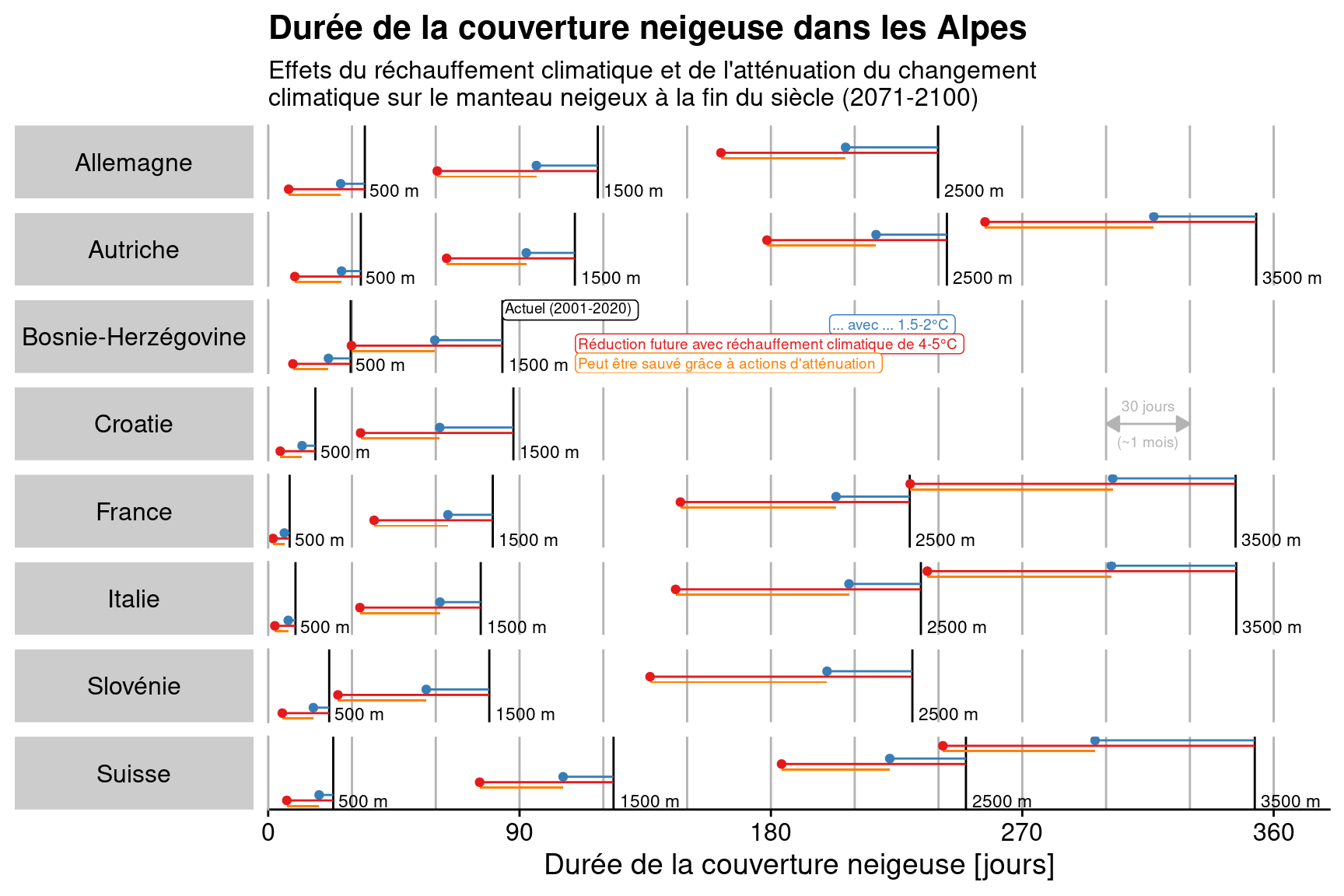
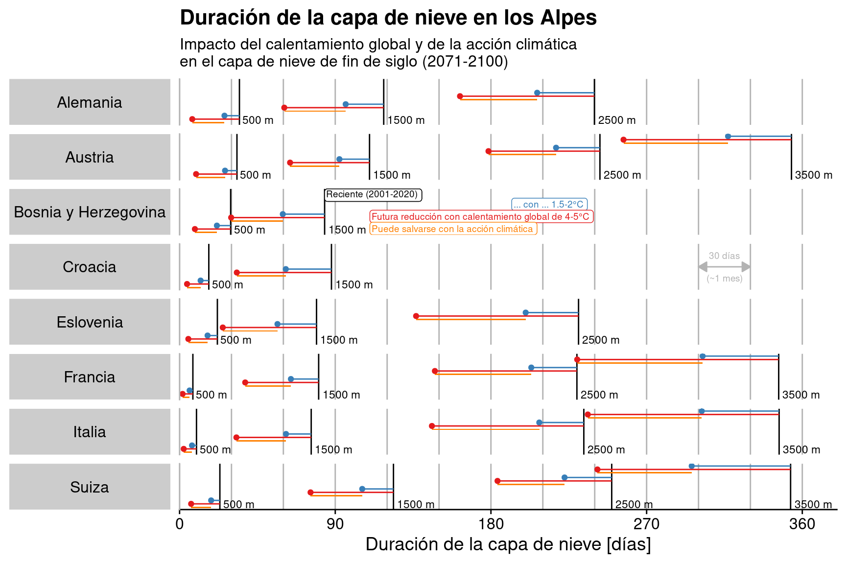
> Overview by countries in the Greater Alpine Region (GAR).

### English

```{r fig.width=9, fig.height=6}


dat_anno_repel <- cbind(dat_anno,
                        yy = 100 + c(1500 + 3.5*dy, 1500, 1500 - 3.5*dy),
                        xx = c(169, 120, 120) - 10,
                        colour = c("rcp26", "rcp85", "loss"),
                        label = c("... with 1.5-2°C warming",
                                  "Reduction in future SCD with 4-5°C warming",
                                  "SCD saved with climate action"),
                        hjust = c(0, 0, 0))


f_plot()
```


### Deutsch


```{r fig.width=9, fig.height=6}


dat_anno_repel <- cbind(dat_anno,
                        yy = 100 + c(1500 + 3.5*dy, 1500, 1500 - 3.5*dy),
                        xx = c(171, 120, 120) - 10,
                        colour = c("rcp26", "rcp85", "loss"),
                        label = c("... mit 1.5-2°C Erwärmung",
                                  "Rückgang in der Zukunft mit 4-5°C Erwärmung",
                                  "Kann mit Klimaschutzmaßnahmen verhindert werden"),
                        hjust = c(0, 0, 0))


f_plot(lang = "DE",
       lbl_month = "Monat",
       lbl_days = "Tage",
       lbl_recent = "Gegenwart (2001-2020)",
       lbl_xlab = "Schneebedeckungsdauer [Tage]",
       lbl_title = "Schneebedeckungsdauer in den Alpen",
       lbl_subtitle = "Einfluss der globalen Erwärmung und der Klimaschutzmaßnahmen \nauf die Schneedecke am Ende dieses Jahrhunderts (2071-2100)")


```

### Italiano


```{r fig.width=9, fig.height=6}


dat_anno_repel <- cbind(dat_anno,
                        yy = 100 + c(1500 + 3.5*dy, 1500, 1500 - 3.5*dy),
                        xx = c(209.5, 120, 120) - 10,
                        colour = c("rcp26", "rcp85", "loss"),
                        label = c("... con ... 1.5-2°C",
                                  "Riduzione futura con un riscaldamento globale di 4-5°C",
                                  "Si può salvare con misure climatiche"),
                        hjust = c(0, 0, 0))


f_plot(lang = "IT",
       lbl_month = "mese",
       lbl_days = "giorni",
       lbl_recent = "Recente (2001-2020)",
       lbl_xlab = "Durata del manto nevoso [giorni]",
       lbl_title = "Durata del manto nevoso nelle Alpi",
       lbl_subtitle = "Impatto del riscaldamento globale e delle misure per l'adattamento \ne la mitigazione sulla copertura nevosa alla fine del secolo (2071-2100)")




```

### Français


```{r fig.width=9, fig.height=6}



dat_anno_repel <- cbind(dat_anno,
                        yy = 100 + c(1500 + 3.5*dy, 1500, 1500 - 3.5*dy),
                        xx = c(211, 120, 120) - 10,
                        colour = c("rcp26", "rcp85", "loss"),
                        label = c("... avec ... 1.5-2°C",
                                  "Réduction future avec réchauffement climatique de 4-5°C",
                                  "Peut être sauvé grâce à actions d'atténuation"),
                        hjust = c(0, 0, 0))


f_plot(lang = "FR",
       lbl_month = "mois",
       lbl_days = "jours",
       lbl_recent = "Actuel (2001-2020)",
       lbl_xlab = "Durée de la couverture neigeuse [jours]",
       lbl_title = "Durée de la couverture neigeuse dans les Alpes",
       lbl_subtitle = "Effets du réchauffement climatique et de l'atténuation du changement\nclimatique sur le manteau neigeux à la fin du siècle (2071-2100)")



```


### Español


```{r fig.width=9, fig.height=6}


dat_anno_repel <- cbind(dat_anno,
                        yy = 100 + c(1500 + 3.5*dy, 1500, 1500 - 3.5*dy),
                        xx = c(202, 120, 120) - 10,
                        colour = c("rcp26", "rcp85", "loss"),
                        label = c("... con ... 1.5-2°C",
                                  "Futura reducción con calentamiento global de 4-5°C",
                                  "Puede salvarse con la acción climática"),
                        hjust = c(0, 0, 0))


f_plot(lang = "ES",
       lbl_month = "mes",
       lbl_days = "días",
       lbl_recent = "Reciente (2001-2020)",
       lbl_xlab = "Duración de la capa de nieve [días]",
       lbl_title = "Duración de la capa de nieve en los Alpes",
       lbl_subtitle = "Impacto del calentamiento global y de la acción climática \nen el capa de nieve de fin de siglo (2071-2100)")



```


### Table (RCP2.6)


```{r}

dat_table <- dat_lollipop[elev %in% c(500, 1500, 2500, 3500)]


dat_table[, value_abs := rcp26_future - rcp26_past]
dat_table[, value_rel := (rcp26_future - rcp26_past) / rcp26_past]
dat_table[, label := sprintf("%2.0f d (%2.0f%%)", round(value_abs), round(value_rel*100, 1))]
dat_table2 <- dcast(dat_table, country_fct ~ elev_fct, value.var = "label")

dat_table2 %>% 
  flextable() %>% 
  set_header_labels("country_fct" = "") %>% 
  set_caption("Global warming 1.5-2°C (RCP2.6)") %>% 
  autofit()

```


### Table (RCP8.5)


```{r}

dat_table <- dat_lollipop[elev %in% c(500, 1500, 2500, 3500)]


dat_table[, value_abs := rcp85_future - rcp26_past]
dat_table[, value_rel := (rcp85_future - rcp26_past) / rcp26_past]
dat_table[, label := sprintf("%2.0f d (%2.0f%%)", round(value_abs), round(value_rel*100, 1))]
dat_table2 <- dcast(dat_table, country_fct ~ elev_fct, value.var = "label")

dat_table2 %>% 
  flextable() %>% 
  set_header_labels("country_fct" = "") %>% 
  set_caption("Global warming 4-5°C (RCP8.5)") %>% 
  autofit()

```




# Maps

## Column

### All maps

Open map of current (2001-2020) average annual snow cover duration (SCD). Click on any point to show associated value. Use layers control on left to toggle between current and future SCD under different greenhouse gas concentration scenarios.


  - RCP2.6 ~ 1.5-2°C global warming
  - RCP8.5 ~ 4-5°C global warming
  

All maps (default 2001-2020) 

  
## Column

### Sliders (present vs. ...)

**{Update June 2022: Possibly not working}**

Open slider with two maps in background comparing the present snow cover duration to the future under different greenhouse gas (GHG) concentration scenarios, the so-called representative concentration pathways [(RCP)](https://en.wikipedia.org/wiki/Representative_Concentration_Pathway).



#### 2041-2070 vs. 2001-2020

1.5-2°C (RCP2.6) 

4-5°C (RCP8.5) 


#### 2071-2100 vs. 2001-2020
  
1.5-2°C (RCP2.6) 

4-5°C (RCP8.5) 




## Column

### Sliders (low vs. high GHG concentrations)

**{Update June 2022: Possibly not working}**

Open sliders with maps in the background that compare the difference between climate action and rising greenhouse gas (GHG) concentrations for two future periods. 

Climate action corresponds to RCP2.6, which is 1.5-2°C of global warming, while rising GHG corresponds to RCP8.5, which amounts to 4-5°C of global warming.

#### Climate action vs. rising greenhouse gas concentrations

2041-2070 

2071-2100